What is a tabular foundation model?
A model that has already learned how to learn from tables. You show it your labeled rows and it predicts new ones in a single forward pass. Nothing gets trained on your data.
A classic model, like logistic regression or XGBoost, starts from zero on every dataset. You fit it to your rows, spend a while tuning it, and when the data changes you go through it all again. A tabular foundation model does its learning once, ahead of time, on millions of synthetic tables built to look like real ones: columns that interact, noisy values, gaps, a class that shows up in only 2% of the rows. It never sees your problem during that training. What it picks up is the general skill of reading a table and working out which columns predict what.
So when you bring your data, nothing gets fitted. Your labeled rows go in as context, the rows you want predictions for go in next to them, and a single forward pass gives back a probability for each class (or a number, if you're doing regression). If you've ever put a few examples in a prompt for a language model, it's the same idea, applied to rows and columns.
Why teams use them
- Much shorter time to production. There's no feature pipeline to tune, no hyperparameter search and no training run to keep an eye on overnight. You bring labeled history, and a few minutes later you have a model you can call and evaluate. The usual route takes weeks.
- Better with every release. Today's models already hold their own against gradient-boosted trees on public benchmarks, and each new generation closes more of the gap that's left. When a better one comes out, your capability picks it up through a new championship, and your integration doesn't change.
- No training to pay for. Since nothing is trained, there are no training runs, tuning sweeps or retraining jobs on the bill. What you pay for is inference.
- Fine-tuning when you need it. The pretrained models work out of the box, and if a use case needs more than that, they can be fine-tuned on your own history.
- A strong model with less ML expertise. Data scientists skip the tuning and spend that time on the actual problem, while a business team can put a good model in production without an ML team behind every use case.
What to expect
- Small data is where they shine. With a few hundred to a few thousand labeled rows, one of these models usually matches or beats a tuned gradient-boosted model, and you didn't tune anything.
- No training pipeline. New history just means new context instead of a new training run, which is why a capability is ready in about a minute.
- Probabilities you can check. They're often close to calibrated out of the box, but that depends on your data, so check them before you build thresholds or expected values on top. Every evaluation includes a calibration curve and the log loss on your holdout (see Metrics).
- Some limits. The context is capped at 10,000 rows here, so a very large history gets sampled. And because every prediction reads the whole context, each one takes more compute than a tree ensemble would.
On your machine, ZeroGrad runs every commercial model you have installed: TabPFN v2 and TabICLv2 come with pip install zerograd, and Mitra-v2 and TabDPT are extras. The platform runs TabPFN v2 and TabICLv2. Either way, every model is scored on a holdout of your data and the one that does better serves your predictions. You'll find the details in Models and licenses.
Quickstart
Here's the whole path from a CSV of labeled history to a classifier you can call. Nothing gets trained along the way. The pretrained models read your examples as context, ZeroGrad tests each one on rows it hasn't seen, and keeps the one that does best. It all runs on your machine with the open source SDK, so you don't need an account or an API key.
pip install zerograd             # TabPFN v2 and TabICLv2
pip install "zerograd[all]" # adds Mitra-v2 and TabDPTimport pandas as pd
from zerograd import ZeroGrad
titanic = pd.read_csv("https://raw.githubusercontent.com/datasciencedojo/datasets/master/titanic.csv")
train, new_passengers = titanic.iloc[:700], titanic.iloc[700:].drop(columns="Survived")
zg = ZeroGrad() # local: runs on your machine, no API key
cap = zg.create("titanic-survival", examples=train, target="Survived")
# prints the championship: every model on the same holdout, the champion on top
cap.evaluation # the same comparison as a DataFrame, champion marked
preds = cap.predict(new_passengers)
# prediction, score, proba_0, proba_1, with the same index as new_passengers
cap.save("titanic.zg") # one file; zerograd.load("titanic.zg") opens it againThe first time a model runs, its weights download from the authors' Hugging Face repository and stay cached for next time. A GPU helps but you don't need one: on a laptop CPU, a history of a few thousand rows takes seconds to a couple of minutes. If you'd rather not install anything yet, the notebooks run the same code in Colab.
On the platform (optional)
When you want ZeroGrad to run it for you, with versions, scheduled championships and monitoring, the same code works against the platform. That's the one part that needs an API key, which you can . Once ZEROGRAD_API_KEY is set, ZeroGrad() picks the platform on its own. Pass remote=False if you want to stay local with the key in your environment.
export ZEROGRAD_API_KEY=zg_live_...zg = ZeroGrad(remote=True) # reads ZEROGRAD_API_KEY and talks to https://api.zerograd.dev
cap = zg.create("titanic-survival", examples=train, target="Survived")
preds = cap.predict(new_passengers)If you'd rather skip the SDK, here's the same thing over plain HTTP:
curl -X POST "https://api.zerograd.dev/v1/capabilities" \
  -H "Authorization: Bearer $ZEROGRAD_API_KEY" \
  -F name=titanic-survival -F target=Survived -F examples=@titanic.csv
# 202 {"capability_id": "cap_9dt5Ls5Cvw", "name": "titanic-survival", "run_id": "run_…", "status": "queued"}

curl "https://api.zerograd.dev/v1/runs/run_…" -H "Authorization: Bearer $ZEROGRAD_API_KEY"
# {"status": "running", "stage": "evaluate", "progress": 0.55, "message": "Running inference with TabICLv2 (2 of 2) · 3,000 / 6,512 holdout rows", …}

curl -X POST "https://api.zerograd.dev/v1/capabilities/titanic-survival/predict" \
  -H "Authorization: Bearer $ZEROGRAD_API_KEY" -H "Content-Type: application/json" \
  -d '{"rows": [{"Pclass": 3, "Sex": "male", "Age": 22, "Fare": 7.25, "Embarked": "S"}]}'
Notebooks
These run end to end in Colab with the open source SDK in local mode, so you don't need an account or an API key. When you want the platform to run them instead, the same code works with ZeroGrad(remote=True).

Use it from an agent (MCP)
The SDK comes with an MCP server, so Claude Code, Cursor, Codex or any other MCP client can use ZeroGrad for you. You ask in plain language, the agent picks the tools, and everything runs on your machine in local mode. You don't need an account or an API key, and none of your data gets uploaded.
pip install "zerograd[mcp]"
claude mcp add zerograd -- zerograd-mcp
If you'd rather not install anything, uvx can run it for you: claude mcp add zerograd -- uvx --from "zerograd[mcp]" zerograd-mcp. Other clients take the same command, zerograd-mcp, over stdio. In Cursor it goes in .cursor/mcp.json, and in Codex in ~/.codex/config.toml:
{
  "mcpServers": {
    "zerograd": { "command": "zerograd-mcp" }
  }
}[mcp_servers.zerograd]
command = "zerograd-mcp"Then just ask. Something like "Predict churn in customers.csv and tell me which columns matter" is enough: the agent looks at the file, creates the capability, predicts and explains, using these tools.
The agent passes file paths around, never the rows themselves, so a big table doesn't have to fit in its context. predict writes <input>.predictions.csv with your columns plus the prediction and score, and hands the agent a summary and a short preview. Capabilities are saved in ~/.zerograd/capabilities (set ZEROGRAD_HOME to move them). They're the same files cap.save() writes, so you can open one in Python with zerograd.load() and keep going from there.
Model weights download from Hugging Face the first time a model runs, as they do in the SDK. The MCP server only uses models you can use commercially, and you'll find the full list in Models and licenses.
If your agent writes the code instead, point it at zerograd.dev/llms.txt. It's an index of these docs in Markdown, and llms-full.txt has all of them in one file, code included. Both are rebuilt from this page on every deploy, so they never fall behind. The SDK repo also has an AGENTS.md for coding agents.
Context size: speed against quality
Every time a foundation model predicts, it reads its whole context, meaning all the labeled rows you gave it. More rows usually buy you a slightly better score, but they always make each answer slower, and past a certain size the score stops improving at all. context_curve helps you find that size. It fits one model on bigger and bigger stratified samples of your context, scores each one on the same test rows and times it. The size it recommends is the smallest one that lands within 0.005 of the best score, and you can change that tolerance.
curve = zg.context_curve(train, "class", test=test)   # sizes: 250, 500, 1K, 2K, 5K, 10K... up to all rows
curve                  # per size: the metric, fit and predict seconds, ms per row; the recommended row marked
curve.recommended      # e.g. 2000
curve.plot()           # score and latency on two axes, the recommended size marked

curve = cap.context_curve(test)                 # the champion, on samples of the capability's own context
cap.update(context_rows=curve.recommended) # predict with the smaller, faster contextwhi). Each size is a stratified sample of 20K labeled rows, scored on the same 1,500 holdout rows. Yours will look different, so run context_curve on your own data.You can pass your own sizes=[...], pick the model with model="tabicl-v2" (by default it uses the first selected model), score with metric="log_loss" or any other metric, and loosen the tolerance with tolerance=0.01. If you don't pass test, it holds out a stratified 20% of the rows and keeps them out of every context. What you get back is a regular DataFrame, so you can export it like any other. With remote=True the curve runs a championship per size on the platform and gives you the same table.
Start from the business problem
Churn, fraud, credit risk, propensity, pricing and segmentation. Each page frames the problem the way you'd scope it at work, says why an in-context model fits it, shows the shortest code that runs on a public dataset, and lists what usually goes wrong before you ship.
Pick your problem
Every page follows the same order: the problem, why a foundation model here, the code, the traps, and what you do with the prediction. The examples run locally with the open source SDK, so you can reproduce them before you bring your own table.
Churn
The model is the easy part. Most of the work is the label: a snapshot date, a horizon (30 days is common), and what counts as leaving. A cancellation, a downgrade and 60 days without logging in are three different targets, and involuntary churn from failed payments usually needs its own model because the fix is different. The output is a ranked list the retention team works from the top.
Why a foundation model here
A churn table is typically a few thousand customers and a few dozen mixed columns: plan, tenure, usage against their own average, tickets. That's the size where an in-context model does well with no tuning, because there's nothing to fit. Your history is the context, and a new snapshot next month is a new context, not a retraining job. churn.baselines scores the same holdout with no model, so you see the gap on your own data instead of taking ours.
import pandas as pd
from zerograd import ZeroGrad

url = "https://raw.githubusercontent.com/IBM/telco-customer-churn-on-icp4d/master/data/Telco-Customer-Churn.csv"
telco = pd.read_csv(url).sample(frac=1, random_state=0)
telco["TotalCharges"] = pd.to_numeric(telco["TotalCharges"], errors="coerce")
history, this_month = telco.iloc[:5_000], telco.iloc[5_000:]

zg = ZeroGrad()                                   # local: nothing leaves your machine
churn = zg.create("churn", examples=history, target="Churn", drop=["customerID"])
churn.evaluation, churn.baselines                 # every model and a no-model baseline, same holdout

risk = churn.predict(this_month.drop(columns=["Churn", "customerID"]))
risk["proba_Yes"]                                 # what you sort by
What usually goes wrong
- Features from after the snapshot. The cancellation reason, a retention call logged the week they left, a "days to contract end" computed today. Build every column as of the snapshot date.
- A random split over snapshots. Stack monthly snapshots and the same customer shows up on both sides of a random split. Validate on later snapshots with
time=, or keep each customer on one side withgroups=. - Unfinished windows. A customer who joined ten days ago hasn't had 30 days to leave. Label only snapshots whose horizon has fully passed, or they count as stayers.
zg.cross_validate(snapshots, "churned", time="snapshot_date", folds=4).summary # train on the past, score the next monthFrom score to decision
If the team's capacity is the constraint, skip the threshold and take the top of the list. If it isn't, put prices on the two mistakes: an offer to someone who'd have stayed costs a discount, a missed churner costs their margin. With a lost customer worth about five offers, the capability picks the cut on the holdout and predicts with it from then on.
churn.optimize_threshold("cost", cost_fp=1, cost_fn=5)       # a lost customer costs 5 offers
call_list = this_month.assign(risk=risk["proba_Yes"]).nlargest(200, "risk")   # or: what the team can call this week
A high risk score doesn't mean an offer will work. Who responds to the offer is an uplift question (see Causal modeling).
Go deeper: Classification · Pick the threshold · Cross-validation by date · Column importance
Fraud
Three things make fraud harder than a regular classifier: the positive rate (under 0.2% in the dataset below), labels that arrive weeks late with the chargeback, and an adversary that changes behavior once you start blocking. A supervised model covers the patterns you've confirmed. Anomaly detection against payments you trust covers the ones you haven't. Most teams run both and route the union to review.
Why a foundation model here
The context holds up to 10,000 rows, so you can put every confirmed fraud in it and sample the legitimate payments around them. The model reads the rare class directly at prediction time instead of having to learn it through class weights. When a new pattern gets labeled, you add those rows to the context and the next prediction already uses them. TabPFN v2 and TabICLv2 also run as anomaly detectors, and tell you which columns make a payment unusual.
import pandas as pd
from sklearn.datasets import fetch_openml
from zerograd import ZeroGrad

cards = fetch_openml("creditcard", version=1, as_frame=True).frame
cards["Class"] = cards["Class"].astype(int)                         # 1 = fraud
fraud, legit = cards[cards["Class"] == 1], cards[cards["Class"] == 0]
sample = pd.concat([fraud, legit.sample(9_500, random_state=0)])   # every fraud, 1 in 30 legit

zg = ZeroGrad()
cap = zg.create("card-fraud", examples=sample, target="Class", drop=["Time"], metric="pr_auc")

found = zg.anomalies(todays_payments, reference=last_month_clean)   # no labels needed
found.top(20)                                                        # the oddest, and the columns behind it
What usually goes wrong
- Immature labels. A payment from last week with no chargeback isn't clean yet. Train only on payments older than your chargeback window.
- Sampling changes the probabilities. With 1 in 30 legitimate payments kept, the scores are inflated against the real base rate. Rank with them, and account for the sampling in the costs (below) or recalibrate before you read them as odds.
- The same card on both sides. Fraud comes in bursts on one card or merchant. A random split puts half a burst in training and makes the holdout look easy. Split by time, or by card with
groups=. - Velocity features that include the payment itself. "Payments in the last hour" has to be computed at authorization time, from what came before. A batch job that counts the whole hour leaks.
From score to decision
A missed fraud costs the amount plus the chargeback fee. A false decline costs a customer at the till, and sometimes the next purchase. Say a miss costs 40 times a false alarm, and remember that each legitimate payment in the sample stands in for 30. If the real limit is how many cases your analysts can review, fix a precision instead.
cap.optimize_threshold("cost", cost_fp=1 * 30, cost_fn=40)    # 30: legit payments sampled 1 in 30
cap.optimize_threshold("recall", min_precision=0.5)            # half of what you flag is real fraud
Go deeper: Predictions and thresholds · Anomaly detection · Why a row is unusual · Outcomes
Credit risk
The model gives a PD for each application. The policy turns it into approve, decline or approve with a lower limit. What makes credit its own problem is the feedback: you learn whether a loan was good months later, and only for the loans you approved. Your training data is shaped by the previous policy, and so is every metric you compute after launch.
Why a foundation model here
Credit portfolios are often small, especially a new product or a new segment, and 1,000 loans is enough to get a usable ranking from an in-context model without a feature engineering cycle first. On a table that small one holdout is noisy, so the example cross-validates before trusting the number, and reads column importance so you can check the model leans on what a credit analyst would expect.
from sklearn.datasets import fetch_openml
from zerograd import ZeroGrad

credit = fetch_openml("credit-g", version=1, as_frame=True).frame
credit["default"] = (credit["class"] == "bad").astype(int)      # 1 = the loan went bad
credit = credit.drop(columns="class")

zg = ZeroGrad()
zg.cross_validate(credit, "default", folds=5).summary            # mean and spread, per model
risk = zg.create("credit-risk", examples=credit, target="default")
risk.importance(credit.sample(300, random_state=1))              # which columns it leans on
What usually goes wrong
- Data you didn't have on the decision date. Anything touched by collections, a bureau pull refreshed after origination, a status field that gets overwritten. It makes the model look brilliant on paper.
- Random split across vintages. Defaults cluster by origination month and by the economy at the time. Validate on later vintages with
time=so the number reflects the loans you'll actually score. - Only approved loans have outcomes. The model never saw how rejected applicants would have done, and the post-launch numbers only cover the people it approved. Keep a small random approval band if your risk appetite allows it.
- Columns you aren't allowed to use. This dataset has personal status and sex in one column. Where you lend, that may be off limits for the decision. The SDK drops what looks like personal data before anything is uploaded (see Privacy and sensitive data), but protected attributes are your call.
From score to decision
This dataset ships with its own cost matrix: approving a loan that goes bad costs five times as much as declining one that would have paid. Use your own loss given default against the margin on a good loan.
risk.optimize_threshold("cost", cost_fp=1, cost_fn=5) # a bad loan approved costs 5 good ones declinedOn the platform every prediction gets an id. Send the outcome back when the loan matures and the platform scores each monthly cohort once its loans have had time to default, recording which ones you approved.
cap = ZeroGrad(remote=True).create("credit-risk", examples=credit, target="default")
cap.update(maturity_days=365)
preds = cap.predict(applications, id_column="application_id")

# a year later
cap.send_outcomes(outcomes_df)        # reference, outcome, decision ("approved", "rejected")
cap.performance(cohort="month")
Go deeper: Pick the threshold · Outcomes · Quality by cohort · Privacy and sensitive data
Propensity and cross-sell
The budget is fixed and the base rate is low, so what matters is how much better the top of the list converts than calling at random. Read lift and precision in the top decile, not overall ROC AUC: two models with the same AUC can rank the first few hundred customers very differently.
Why a foundation model here
Campaign tables change every time. A new product, a new channel or a new segment means a new target with little history, and an in-context model gives you a ranked list from the last campaign without a modeling cycle in between. cross_validate reports lift in the top 10% for every model next to a baseline, which is the number to take to whoever owns the budget.
from sklearn.datasets import fetch_openml
from zerograd import ZeroGrad

bank = fetch_openml(data_id=46910, as_frame=True).frame.sample(8_000, random_state=0)
history, next_campaign = bank.iloc[:6_000], bank.iloc[6_000:]

zg = ZeroGrad()
zg.cross_validate(history, "SubscribeTermDeposit", folds=3).summary   # lift in the top 10%, per model
buy = zg.create("term-deposit", examples=history, target="SubscribeTermDeposit")

scores = buy.predict(next_campaign.drop(columns="SubscribeTermDeposit"))
shortlist = next_campaign.assign(p=scores["proba_yes"]).nlargest(400, "p")
What usually goes wrong
- Columns that only exist after contact. In the original version of this dataset the call duration predicts the sale almost perfectly, and you only know it after hanging up. The version above leaves it out.
- Last campaign's targeting is in the label. If an earlier model chose who got called, the history only shows outcomes for the people it liked. Customers it skipped look like non-buyers because nobody asked.
- A loose window. Fix the window per campaign. A purchase three months later through another channel is probably not this campaign's sale.
- Propensity isn't uplift. The top of the list includes people who'd have bought anyway. If the goal is to spend only where the call changes the outcome, that's uplift modeling (see Causal modeling).
From score to decision
With a fixed budget, sort and stop where the money runs out. Without one, price the two mistakes: a call that doesn't sell against a sale you never asked for. If a sale is worth about eight calls, let the cost pick the cut.
buy.optimize_threshold("cost", cost_fp=1, cost_fn=8) # a sale is worth 8 callsGo deeper: Classification · Cross-validation · Pick the threshold · Causal modeling
Pricing and demand
Two related problems. Valuation predicts what a unit is worth from its attributes, the way a hedonic model would: location, size, condition. Demand predicts how much sells given the context: day, season, weather, promotion, price. Both read each row's own columns, which is what separates them from forecasting a single series from its own past.
Why a foundation model here
Pricing data has a long tail: plenty of rows for common items and very few for the rest. An in-context model handles new and rare items through their attributes, without a history of their own, which a per-series model can't do. value.baselines scores the average and the median on the same holdout, so you know what the model adds before anyone uses its prices.
from sklearn.datasets import fetch_california_housing, fetch_openml
from zerograd import ZeroGrad

zg = ZeroGrad()

# valuation: median house value of a block, in $100,000
houses = fetch_california_housing(as_frame=True).frame.sample(5_000, random_state=0)
value = zg.create("house-value", examples=houses.iloc[:4_000], target="MedHouseVal", metric="mae")
value.evaluation, value.baselines

# demand: rentals per hour, the last 1,000 hours held out as the future
bikes = fetch_openml("Bike_Sharing_Demand", version=2, as_frame=True).frame
demand = zg.create("bike-demand", examples=bikes.iloc[:-1_000], target="count", drop=["casual", "registered"])
demand.predict(bikes.iloc[-1_000:].drop(columns=["count", "casual", "registered"]))
What usually goes wrong
- Components of the target. The bike data counts casual and registered riders separately, and the two sum to the total. Same story with units sold split by channel. They have to go.
- Interpolating instead of predicting. A random split over hourly data lets the model see 2 p.m. and 4 p.m. while you score 3 p.m. Hold out the last stretch, as above, or cross-validate with
time=. - Reading elasticity off observed prices. Prices went up when demand was high, so a model on historical data learns the correlation, not what a price change will do. To set a price you need variation that demand didn't cause, like a test or a staggered rollout.
- A target that spans orders of magnitude. Predict the log of the price and the error becomes relative, so a $50 miss on a $100 item and on a $10,000 item stop counting the same.
From prediction to decision
There's no threshold here. The choice is which error you're paying for. If every unit off costs the same, select by MAE, which reads in the target's unit: an MAE of 0.3 here means the typical block is off by about $30,000. If large misses hurt more, like running out of stock on a Saturday, select by RMSE. Either way, the holdout error is the first estimate of the margin you keep around a reference price or a stock level.
If what you have is a sales history per product and you want the next few weeks, that's forecasting, which is on the way (see Forecasting).
Go deeper: Regression · Regression metrics · Cross-validation by date · Forecasting
Customer segments
No target, so there's no single number that says you're done. A segmentation is good when it's stable, when each segment behaves differently on something you can act on, and when the people using it can describe each group in a sentence. Most of the decisions are in the columns you feed it.
Why a foundation model here
cluster runs ZEUS, a zero-shot clustering model, next to k-means and a Gaussian mixture, and picks the number of segments for you. If you have a label you trust, like the channel below, pass it as labels= to score every method against it. It's never read as a feature.
import pandas as pd
from zerograd import ZeroGrad

url = "https://archive.ics.uci.edu/ml/machine-learning-databases/00292/Wholesale%20customers%20data.csv"
shops = pd.read_csv(url)                         # yearly spend on fresh, milk, grocery, frozen...

zg = ZeroGrad()
segments = zg.cluster(shops.drop(columns=["Channel", "Region"]))   # k between 2 and 10
segments.profiles                                # size and what sets each segment apart
zg.cluster(shops.drop(columns="Region"), labels="Channel").evaluation   # does it recover hotels vs retail?
What usually goes wrong
- Size splits. Spend columns are skewed and correlated with how big the customer is. Fed raw, they give you small, medium and large. Use shares of spend or logs if behavior is what you're after.
- Clusters always come out. Every method returns groups, even from noise. Rerun on a different sample and check that customers land in the same segment before anyone builds a campaign on it.
- Identifiers and outcomes in the input. IDs and free text are dropped for you. Columns like churn or revenue next quarter are better used to describe segments afterwards than to form them.
Choosing how many
The SDK picks the number that separates best, but the right number is also the one your team can work with. Try k=3, k=4 and k=5, read the profiles, and keep the split where each segment gets a name and an action.
Go deeper: Clustering · Without a target
Capabilities
A capability is one prediction your product makes, like whether a customer is about to churn or what a listing will sell for. Behind it sits your labeled history, and in front of it, the foundation model that did best on that history. This part covers what every capability has in common. The sections after it cover what each type adds.
How it works
When you create a capability, Zero Grad runs a championship. Every model that can handle the capability's type gets the same context and is scored on the same holdout rows, and whichever gets the best value of the capability's metric becomes the champion. Here's what happens, in order:
- The columns are profiled, and the ones that can't help are dropped.
- 20% of the labeled rows (at most 20,000) are held out, stratified on the target: by class, or by deciles if the target is a number. Every model scores every one of these rows.
- The rest become the context. If there are more than 10,000, a sample of 10,000 is taken, stratified the same way.
- A few baselines are scored on the same holdout, so you can see how much a model adds over a guess.
- The champion is picked, and it keeps a context drawn from all the labeled rows for predictions.
- The champion is warmed up, so your first predictions after create come back fast.
| Classification | A category: churn, fraud, default. Binary or multiclass, up to 10 classes. | SDK and platform |
| Regression | A number: a price, a demand, a time to resolve. | SDK |
Which foundation model sits behind a capability is an implementation detail. If a tournament later finds a better champion, it takes over and your integration stays exactly as it was.
Create a capability
A capability is a name, the history behind it and the versions that serve it. You don't have to tell it the type, because it reads that from the target column. Categories, true/false and whole numbers with up to 10 distinct values make a classification. Numbers with decimals, or with more distinct values, make a regression. If you'd rather say it yourself, pass task=.
import zerograd
from zerograd import ZeroGrad

zg = ZeroGrad()
cap = zg.create(
    "churn",                            # the name: lowercase letters, digits and dashes
    examples="customers.parquet",       # a DataFrame or a CSV/Parquet path
    target="churned",
    drop=["cancellation_reason"],       # columns only known after the outcome
    metric="pr_auc",                    # how the champion is picked (each type has its default)
    task="classification",              # optional: "classification" or "regression"
)

cap.evaluation                          # every model's metrics on the same holdout; the champion is marked
cap.baselines                           # the same holdout scored without a model
cap.save("churn.zg")                    # one file with the context, no weights
cap = zerograd.load("churn.zg")         # open it again, in this process or another one

# on the platform, with ZeroGrad(remote=True)
zg.capabilities()                       # list
cap = zg.capability("churn")            # by name or id
cap.delete()                            # capability, versions and stored history
What happens to your data
Before anything runs, the columns that can't help are dropped: identifiers, free text, and columns that are constant or empty. Each one shows up in dropped_columns with the reason, and you can drop more yourself with drop=[...]. Numbers, booleans, dates and categories are encoded for you. If a category shows up later that wasn't in the history, it's treated as missing.
The capability lists its expected_columns. Predictions need those columns, and any extra ones you send are ignored. Locally, nothing leaves your machine. On the platform, your history is stored in your workspace and deleted together with the capability, and examples can also be a gs:// URI or an upload id.
Metrics
Every model is scored on the holdout with all the metrics for the capability's type, and one of them decides the champion. You choose which with metric=, and tournaments and context curves use that same one. If you don't choose, it's ROC AUC for classification and RMSE for regression. Asking for a metric that doesn't fit the type gets you an invalid_metric error.
Versions
On the platform, if you create a capability with a name that already exists, you get a new version of it, and that version becomes the current one. To predict against an older version, pass version=1. Locally, each file you save is its own version, so keep the ones you want to go back to.
Predict
preds = cap.predict(new_rows)           # DataFrame aligned to the input's index
cap.predict({"plan": "pro", "tenure": 14})   # one row as a dict returns a dict
Locally, the champion scores your rows in chunks, however many you send. On the platform, how the request is handled depends on how much you send:
Every prediction comes with a prediction. What else you get depends on the type. Classification adds probabilities and a threshold, while regression gives you just the number.
Evaluate and decide
The championship tells you which model did best on one holdout. Before a capability goes to production you'll usually want to know a bit more. Does the result hold up on other splits? Where should a binary score draw the line? Which columns is it leaning on? The tools below answer those questions, and they run with the open source SDK on your own machine.
Cross-validation
cv = zg.cross_validate(df, "default", folds=5)                  # stratified k-fold
cv = zg.cross_validate(df, "default", groups="customer_id")     # a customer never sits on both sides
cv = zg.cross_validate(df, "default", time="date", gap=30)      # train on the past, score the next block
cv.summary      # per model: mean metrics, spread, KS and lift in the top 10%, next to a baseline
cv.folds        # one row per model and fold
cv.best
A random split can flatter a model. If the same customer shows up on both sides, the model gets credit for recognizing them, and if rows from next month land in the context, it gets to peek at the future. So when rows repeat per customer, store, patient or device, split by group, and when the capability will predict what comes next, split by time. The group and time columns are left out of the features, and each fold's context is a stratified sample of its training rows.
Pick the threshold
cap.optimize_threshold("cost", cost_fp=1, cost_fn=20)    # a missed default costs 20 false alarms
cap.optimize_threshold("recall", min_precision=0.8)      # catch the most while 8 in 10 flags are right
cap.optimize_threshold("f1", apply=False).table          # precision, recall, cost and share flagged per cut
This works on binary capabilities. It reads the confusion counts the championship already saved for every cut from 0.01 to 0.99, so it doesn't need new predictions, and it sets the capability's threshold for you unless you pass apply=False. You can optimize for f1, cost, youden, recall with min_precision, and precision with min_recall. To work from other rows instead, pass them with the target as data=.
Column importance
cap.importance(test_df) # how much the metric drops when each column is shuffledYou pass some rows with the target, and each column gets shuffled in turn. How much the capability's metric drops is that column's importance, so a column near zero is one you could probably drop. Use rows the model didn't read as context, or the numbers will come out too optimistic.
scikit-learn
If you already work with scikit-learn, you can use a foundation model as one more estimator, next to a random forest or a logistic regression. ZeroGradClassifier and ZeroGradRegressor have the usual fit, predict and predict_proba, so they go anywhere a scikit-learn model goes: a Pipeline, cross_val_score, GridSearchCV, TunedThresholdClassifierCV or permutation_importance.
from zerograd import ZeroGradClassifier, ZeroGradRegressor
from sklearn.ensemble import HistGradientBoostingClassifier
from sklearn.model_selection import cross_val_score

tfm = ZeroGradClassifier(model="tabicl-v2")   # or leave model out: the first one installed
gbm = HistGradientBoostingClassifier()          # what you use today

cross_val_score(tfm, X, y, cv=5, scoring="roc_auc").mean()
cross_val_score(gbm, X, y, cv=5, scoring="roc_auc").mean()   # same folds
There's one thing that works differently. With a foundation model, fit doesn't train anything. It keeps your rows (a stratified sample of up to 10,000) as the context, and predict hands that context to the model together with the new rows. So fit is quick and predict is where the work happens. Columns get the same cleanup as in a capability: categories, booleans and dates are encoded, and identifiers, free text and constant columns are left out.
When should you use this instead of a capability? A capability runs a championship, picks the best model for you and gives you evaluation, thresholds and saving on top. The estimators skip all of that: you choose the model, and scikit-learn does the comparing. Reach for them when you want to benchmark a foundation model against what you already have, or plug it into a pipeline you already run.
Classification
Use it when the answer is a category: will this customer churn, is this payment fraud, will this loan default. It handles binary and multiclass targets with up to 10 classes, both in the SDK and on the platform.
Overview
Used for: churn, fraud, credit risk, propensity and cross-sell
If your target has categories, true/false values or up to 10 different whole numbers, it's a classification. Every installed commercial model gets to compete: TabPFN v2, TabICLv2, Mitra-v2 and TabDPT when you run locally, and the platform's models with remote=True. If two models tie, the one with the lower log loss wins. The baselines are random scores and always predicting the most common class.
Metrics
For a binary capability you get ROC AUC, PR AUC, log loss, accuracy, balanced accuracy, F1, precision and recall. For multiclass you get ROC AUC, log loss, accuracy, balanced accuracy and macro F1. ROC AUC picks the champion unless you choose another one. The evaluation also includes the confusion matrix, and on binary targets you get the ROC and precision-recall curves as well, plus the confusion counts at every threshold from 0.01 to 0.99.
whi). 5,000 rows of context. The dashed lines are what a coin flip would get: the diagonal for ROC, the share of positives (37%) for precision.whi). Holdout rows grouped into ten score bins (bins with fewer than 10 rows left out); each point is a bin's average score against the share that was actually positive. The dashed diagonal is perfect calibration. Your data may look different, and every evaluation includes this curve for your own holdout.Predictions and thresholds
{
  "capability_id": "cap_9dt5Ls5Cvw",
  "version": 1,
  "model": "tabpfn-v2",
  "classes": [0, 1],
  "predictions": [
    {"prediction": 0, "score": 0.11, "proba": {"0": 0.89, "1": 0.11}}
  ]
}
score is the probability of the positive class, so you only see it on binary capabilities. Multiclass predictions come with prediction and proba.
On a binary capability, prediction is simply score >= threshold, and the threshold is 0.5 until you change it. You can set it once on the capability, override it for a single call, or ignore it and work with the probabilities directly:
cap.update(threshold=0.3)              # from now on, score >= 0.3 predicts the positive class
cap.predict(df, threshold=0.7)          # just this call
cap.update(threshold=None) # back to 0.5whi). Same holdout as above. Counts at each threshold come from the evaluation (thresholds), so moving the slider doesn't retrain anything.Regression
Use it when the answer is a number, like what a listing will sell for or how long a ticket will take to close. Regression runs with the open source SDK on your own machine. On the platform, capabilities are classification only for now.
Overview
Used for: pricing and demand
A numeric target with decimals, or with more distinct values than classification allows (10), is treated as a regression. You can also say so with task="regression", or go the other way with task="classification" for a numeric label like a 1 to 5 rating. The championship works the same. The one difference is that the holdout and the context are stratified on deciles of the target, so both get cheap rows and expensive ones. The baselines are always predicting the average and always predicting the median of the context.
| TabPFN v2 | tabpfn-v2 | Its own regressor checkpoint (Prior-Labs/TabPFN-v2-reg), same license: show Built with PriorLabs-TabPFN. |
| TabICLv2 | tabicl-v2 | Regressor checkpoint tabicl-regressor-v2. BSD-3-Clause. |
| TabDPT | tabdpt | The same checkpoint as classification. Apache 2.0, with pip install "zerograd[tabdpt]". |
All three run on CPU and are on by default once installed. Mitra-v2 doesn't compete in regression yet, because its regressor needs a fine-tune on a GPU. To see which models run each type, call zerograd.list_tasks().
from zerograd import ZeroGrad

zg = ZeroGrad()                         # local: runs on your machine, nothing leaves it
cap = zg.create("listing-price", examples="listings.parquet", target="price", metric="mae")
cap.evaluation                          # RMSE, MAE and R² per model; the champion is marked
If the target has values that aren't numbers, you'll get non_numeric_target. In this version regression capabilities only run locally, so ZeroGrad(remote=True) refuses task="regression" with unsupported_task.
Metrics
Every model reports RMSE, MAE and R² on the holdout. The first two are in the target's own unit, so an MAE of 12,000 on listing prices means the model is off by 12,000 on average. RMSE picks the champion unless you pass metric="mae", which cares less about a handful of big misses, or metric="r2". Always look at the baselines too: if a model can't beat predicting the average every time, it isn't learning anything from your columns. Each model's evaluation also includes predicted against actual for a sample of holdout rows, and a histogram of the errors.
Predictions
preds = cap.predict(new_listings)       # one column: prediction
cap.predict({"size_m2": 80, "rooms": 3, "hood": "norte", "age": 12})
# {"prediction": 154230.5}
There's no score, probability or threshold here. prediction is the number itself, and passing a threshold to a regression capability is an error.
Context size
Context curves work the same way here, with one difference in the tolerance. RMSE and MAE are in the target's unit, so a fixed 0.005 would mean nothing for prices in the hundreds of thousands. For those two the tolerance is relative, and the recommended size is the smallest context within 0.5% of the best error. R² keeps the absolute 0.005.
curve = zg.context_curve(listings, "price", test=holdout)   # RMSE per size, with fit and predict times
curve.recommended                                           # e.g. 2000
cap.update(context_rows=curve.recommended) # predict with the smaller, faster contextForecasting
Predict where one or many time series go next from their history, using time series foundation models, with prediction intervals around each value.
Examples. Weekly demand per SKU, cash flow, call volume, energy load.
It will work like the other capability types, with create and predict, in the SDK and on the platform. If you'd like to try it on your data first, .
Causal modeling
Estimate how much an action changes the outcome for each row: how much a discount, a call or a reminder moves that particular customer. This is uplift, or treatment-effect, modeling, and it tells you who is worth acting on and who would have bought, paid or stayed anyway.
Examples. Who should get a retention offer, which overdue accounts are worth a call, which promotions actually move sales.
It will work like the other capability types, with create and predict, in the SDK and on the platform. If you'd like to try it on your data first, .
Marketing mix modeling
Work out how much each marketing channel adds to sales from your weekly spend and results, including where extra money stops paying off, and see how the same budget could be split to get more out of it.
Examples. TV, search and social budgets, returns per channel, planning next quarter's spend.
It will work like the other capability types, with create and predict, in the SDK and on the platform. If you'd like to try it on your data first, .
Recommendations
Rank the items each user is most likely to want next, from their history and from what people like them did. You send the user and a set of candidates, and you get them back in order with a score each, so you can show the top few or pick the next best offer. New users and new items get a sensible ranking from their attributes alone, before there's any history to go on.
Examples. Products to show on a home page, the next offer for each customer, articles or videos to suggest, which leads a salesperson should call first.
It will work like the other capability types, with create and predict, in the SDK and on the platform. If you'd like to try it on your data first, .
Anomalies, gaps, synthetic rows and segments
Four tasks that don't need labels. They run with the open source SDK on your own machine. Whenever there's something to measure, each one puts the foundation models next to the classic scikit-learn method, so you can see what the model actually adds.
How it works
A tabular foundation model that can classify can also tell you how likely an entire row is. The trick is to split the row's probability into one question per column: how likely is this value, given the columns before it? Each of those questions is a classification the model answers in one forward pass, with your rows as the context, and averaging over a few column orders keeps the result stable. This is the method from the TabPFN paper. The SDK implements it for any classifier, which is how TabPFN v2 and TabICLv2 detect anomalies, fill gaps and generate rows. Two other models are built for a single task each and run zero-shot.
| TabPFN v2 | tabpfn-v2 | Anomalies, imputation, synthetic data | Prior Labs License (Apache 2.0 with attribution): show Built with PriorLabs-TabPFN. |
| TabICLv2 | tabicl-v2 | Anomalies, imputation, synthetic data | BSD-3-Clause. |
| FoMo-0D | fomo-0d | Anomalies | MIT. Zero-shot outlier detection (CMU, ICML 2025), up to 100 features. |
| ZEUS | zeus | Clustering | Apache 2.0. Zero-shot embeddings for clustering (Jagiellonian University, 2025). |
All of them allow commercial use. Columns are profiled just like for a capability, so identifiers, free text, and constant or empty columns are dropped and reported. On the platform these tasks are part of Zero Grad Labs for design partners, and ZeroGrad(remote=True) refuses them with local_only.
Anomaly detection
Used for: fraud
Every row gets a score and the most unusual ones are flagged. With the foundation models you also find out which columns make each of those rows stand out.
from zerograd import ZeroGrad

zg = ZeroGrad()
found = zg.anomalies(transactions)              # cross-fitted: no row is scored against itself
found.top(10)                                    # the 10 most unusual rows, their values and why
found.scores                                     # anomaly_score, percentile, is_anomaly, why
zg.anomalies(today, reference=last_month)        # score new rows against rows you trust
zg.anomalies(transactions, labels="fraud")       # known cases: a championship by ROC AUC
Without labels, the first one available out of TabPFN v2, FoMo-0D and TabICLv2 does the scoring, and the top 5% gets flagged (change that with contamination=). If you have a column of known cases, say transactions you already know were fraud, every foundation model competes with Isolation Forest, Local Outlier Factor and kNN distance on ROC AUC and PR AUC, and the champion scores your rows.
Why a row is unusual
Because the row's probability is built column by column, each column gets its own surprise: how unlikely its value was, given the rest of the row. The why column names up to three columns that are far more surprising than usual for that column, like an income that doesn't fit the person's age and segment. FoMo-0D and the classic methods give you a score but no reason.
Imputation
This fills the missing values in a table, but first it checks which method fills them best. In every column with gaps we hide 10% of the values you do have (up to 300 per column), let each method fill them in, and measure how close it got. Then the winner fills the real gaps.
filled = zg.impute(customers)
filled.evaluation                       # error per method and per column; lower is better
filled.data                             # your table with the gaps filled, same index and columns
filled.filled                           # True where a value was filled in
Numbers are scored by RMSE divided by the column's spread, where 0 is perfect and 1 is no better than guessing the mean. Categories are scored by error rate. TabPFN v2 and TabICLv2 predict each column from all the others, using their regressors for numbers, and they compete against mean and mode, KNN and iterative imputation. If your table has no gaps, you'll get nothing_to_impute.
Synthetic data
This makes new rows with the same columns and the same relationships as yours. That's handy for testing a pipeline, sharing examples with someone, or getting more rows of a rare case. Each generator is scored by how hard its rows are to tell apart from your real ones.
fake = zg.synthesize(customers, n=5_000)
fake.data                               # the new rows, with your column types and categories
fake.evaluation                         # detection_auc (0.5 = indistinguishable) and exact_copies
The models build each row one column at a time. For every column they draw a range from what the earlier columns predict, then pick a real value from that range, so your formats stay intact. Then a classifier tries to tell the synthetic rows from the real ones. The generator that gets closest to 0.5, where the classifier is just guessing, wins, and the baseline it has to beat samples every column on its own. Keep in mind that synthetic rows aren't anonymous by themselves. Check exact_copies and drop identifying columns before you share them.
Clustering
Used for: customer segments
Group your rows into segments and see what sets each one apart.
groups = zg.cluster(customers)          # k between 2 and 10, the one that separates best
groups = zg.cluster(customers, k=4)     # or say it
groups.labels                           # the segment of each row
groups.profiles                         # rows, share and what sets each segment apart
zg.cluster(customers, labels="plan")    # known groups: scored by adjusted Rand index
ZEUS embeds up to 2,000 rows at once, zero-shot, and k-means groups those embeddings. The rest of your rows join whichever segment they're closest to. It competes with k-means and a Gaussian mixture run on your standardized columns, and you see the silhouette of each. If you pass known groups, the best adjusted Rand index wins. Without them, the foundation model is the default.
The managed platform for foundation-model ML
Everything so far runs with the open source SDK on your own machine. The platform runs it for you instead, with managed GPU inference and SLAs, championships that rerun on a schedule as new history comes in, and versions, deployments and monitoring. Your code stays the same: set your API key and switch to ZeroGrad(remote=True).
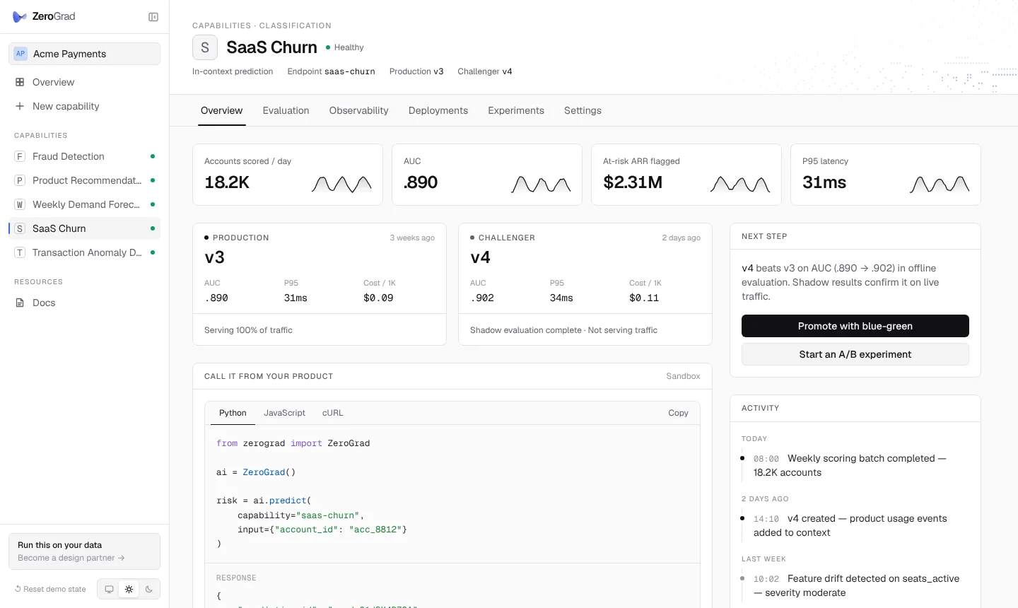
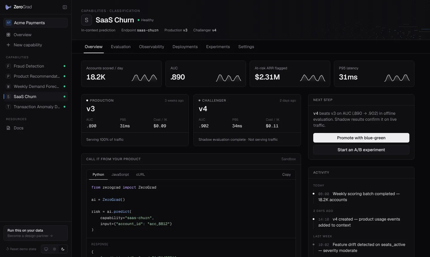
A demo workspace with simulated data: nothing in it calls a model.
Overview
See it →All your capabilities in one place, each with its status, traffic, quality and latency, the version in production and what to do next.
Evaluation
See it →The championship in full: every model on the same holdout, the ROC and precision-recall curves, the confusion matrix, what each threshold trades off, and the result explained in plain language.
Observability
See it →Requests, rows, latency (p50, p95, p99) and errors hour by hour, measured against an availability and latency SLO.
Deployments
See it →One version serves all the traffic. You can promote any version or roll back in one click, and every switch is logged.
Experiments
See it →Tournaments, where the serving champion faces a fresh championship on new history. The challenger only gets promoted if it wins by the margin you set.
Pipelines and runs
Scheduled tournaments and batch scoring from Cloud Storage, with the stages, log and output of every run.
Integrate
The call in Python, JavaScript or curl, a request you can edit and run right there, and a SKILL.md for agents.
Settings and usage
See it →The selection metric and decision threshold of each capability, and for the workspace, rows per day, budgets, alerts and a hard stop.
The sections below cover the API side of the platform, which works the same for every task: runs, large files, privacy and pipelines. In their examples, zg is ZeroGrad(remote=True) with ZEROGRAD_API_KEY set.
Runs
Anything that takes more than a few seconds becomes a run: creating a capability, large predictions and pipelines. The request answers right away with a 202 and a run_id. You can poll it, or let the SDK wait for you.
run = cap.predict("gs://acme-zg/incoming/2026-11.parquet", wait=False)
run            # <Run run_9cT1 predict running 12% · Scoring 31,420 rows with TabPFN v2>
run.wait()
run.output()   # DataFrame with the predictions
run.cancel()   # stops between stages
A run goes queued → running → succeeded, or ends as failed or canceled. A failed run carries the same error body you'd get from a failed request.
Large files
The SDK sends anything over 10 MB through a resumable session in 8 MB chunks, so if your connection drops halfway, the upload picks up where it left off. Over HTTP you do the same by hand: create a session, PUT the chunks with Content-Range, and then pass the upload_id.
# automatic: any DataFrame or file over 10 MB goes through a session
zg.create(name="churn", examples="history-2026.parquet", target="churned")

# or upload once and reuse the id
with open("history-2026.parquet", "rb") as f:
    upload_id = zg.upload(f.read(), "history-2026.parquet")
zg.create(name="churn", examples=upload_id, target="churned")
If your data is already in Cloud Storage, you don't need to upload it. Pass a gs:// file, folder or glob as examples, as the input to a prediction or as a pipeline source, and it's read where it is.
Privacy and sensitive data
The SDK has two tools that keep sensitive data on your side. Both run on your machine before anything is sent, so whatever they remove or hide never reaches ZeroGrad.
Personal data is dropped by default
create and predict look for columns that hold personal data. They check each column's name (email, phone, dni, cuit, ssn, passport, iban, card number, address, birth date, name…) and what's inside it (email addresses, phone numbers, card numbers that pass the Luhn check, CUIT/CUIL, IP addresses). Any column that matches is dropped, and you get a SensitiveDataWarning that names each one and says why.
cap = zg.create(name="churn", examples=df, target="churned")
# SensitiveDataWarning: Dropped before upload: 'email' looks like email (by its values);
#   'customer_name' looks like person name (by its name).

zg.create(..., keep=["zip_code"])      # this one is fine to send
zg.create(..., sensitive="warn")       # warn only, send everything
zg.create(..., sensitive="keep")       # skip the check

from zerograd import scan, drop_sensitive  # the same check, on its own
scan(df)                                   # [Finding(column='email', kind='email', why='content'), ...]
Pseudonymise everything with your own key
A Vault swaps column names, categories and the target's labels for tokens made from a key that only you hold. Numbers go through a linear map derived from the same key. Since the same value always turns into the same token, the models learn exactly as they would on the original data. Predictions come back decoded, with your own labels, column names and index.
from zerograd import ZeroGrad, Vault

key = Vault.new_key()              # once; keep it like a password (a secret manager, an env var)
vault = Vault(key)

cap = zg.create(name="churn", examples=df, target="churned", vault=vault)
preds = cap.predict(new_rows, vault=vault)   # prediction and proba_<label> in your labels

# in another process: the same key, plus the labels (or vault.save / vault.load)
vault = Vault(os.environ["ZEROGRAD_VAULT_KEY"])
preds = vault.decode(raw_preds, labels=[0, 1], target="churned")
On Titanic, the same split scored a ROC AUC of 0.879 without a vault and 0.880 with one. That's expected, because tabular foundation models normalise each column anyway, so the keyed map doesn't touch anything they rely on.
Keep in mind that a vault pseudonymises your data. It doesn't encrypt it. Names and values are hidden, but what the model needs is still there: how often each category appears, the order of the numbers, how columns move together. Use one key per capability for its whole life, because predicting with a different key sends tokens the capability has never seen. And if a column must not leave your side in any form, drop it.
Pipelines
A pipeline repeats a piece of work, either on a schedule (cron, in UTC) or whenever you run it. There are two kinds.
# re-elect the champion on fresh history; promote only on a real gain
cap.pipelines.create(
    kind="tournament",
    source="gs://acme-zg/churn/history/",
    schedule="0 6 * * 1",                      # Mondays 06:00 UTC
    promote_if="roc_auc >= champion + 0.005",
)

# score every new file with the champion
pipe = cap.pipelines.create(
    kind="batch",
    source="gs://acme-zg/incoming/*.parquet",
    output="gs://acme-zg/predictions/",
    schedule="0 2 * * *",
)
pipe.run()                                     # run once now
A tournament scores the current champion and the challengers on the same holdout, and only adds a new version if a challenger wins by the margin in promote_if. A batch pipeline scores every file it hasn't seen yet and writes <name>.predictions.parquet to output.
Outcomes
Used for: credit risk, fraud
The holdout tells you how good a model was on the day it was chosen. To know how it does in production, you need what actually happened to the rows it scored, and that usually arrives much later. A loan you score today defaults, or doesn't, in three or six months. So you send those outcomes back, and the platform puts them next to the predictions they belong to.
Every prediction comes back with a prediction_id. If you'd rather use your own ids, pass id_column and the value of that column is kept as the prediction's reference. You can send outcomes by either one.
preds = cap.predict(applications, id_column="loan_id")
preds[["prediction_id", "score"]]          # same index as applications

# months later, from your own systems
cap.send_outcomes([
    {"reference": "L-10293", "outcome": 1, "decision": "approved", "observed_at": "2027-02-11"},
    {"reference": "L-10294", "decision": "rejected"},     # it will never have an outcome
])
# {'received': 2, 'matched': 2, 'unmatched': 0, ...}

cap.send_outcomes(outcomes_df)             # a DataFrame or a Parquet/CSV file works too
An outcome is one of the capability's classes. A decision is whatever you did with the prediction (approved, rejected, called, sent a discount), as free text. Sending the same id again updates it, so you can send the decision first and the outcome later. Outcomes don't count towards your rows.
We keep the ids, the scores, the version and the time of each prediction, and never the columns you sent to get it. Deleting the capability deletes all of it.
Quality by cohort
Predictions are grouped by the day, week or month they were made. A cohort only counts once its outcomes have had time to happen, which you set per capability with maturity_days. With 90 days, the loans scored this week get metrics 90 days after the week ends. Before that, a loan that hasn't defaulted yet would look like a good loan, and the numbers would look better than they are.
cap.update(maturity_days=90)

perf = cap.performance(cohort="week")
perf[["predictions", "with_outcome", "coverage", "mature", "roc_auc"]]
perf.attrs["by_version"]   # each version in production against its holdout score
Comparing each version with the score it had on the holdout is the simplest way to see drift. If a version that scored 0.86 there is at 0.79 on mature cohorts, the data it sees has changed, and it's time for a tournament on fresh history.
One thing this doesn't solve on its own: you only see outcomes for the cases you acted on. A rejected loan never gets the chance to default, so the metrics only cover the ones you approved. That's why each cohort shows how many predictions have an outcome, split by decision, so you can see how big that gap is. Correcting for it, with reject inference or a control group, depends on how each business decides, and on Platform + FDE and Enterprise our engineers model it with you.
Reference
Models and licenses, errors, limits, every endpoint, and what's coming next.
Models and licenses
| TabPFN v2 | tabpfn-v2 | Prior Labs License (Apache 2.0 with attribution): show Built with PriorLabs-TabPFN. | SDK and platform |
| TabICLv2 | tabicl-v2 | BSD-3-Clause. | SDK and platform |
| Mitra-v2 | mitra-v2 | Apache 2.0. Classification, with pip install "zerograd[mitra]". | SDK |
| TabDPT | tabdpt | Apache 2.0. Classification and regression, with pip install "zerograd[tabdpt]". | SDK |
| Mitra | mitra | Apache 2.0. The first version, only when you name it. | SDK |
| FoMo-0D | fomo-0d | MIT. Anomaly detection. | SDK |
| ZEUS | zeus | Apache 2.0. Clustering. | SDK |
All of these allow commercial use, and ZeroGrad hosts none of the weights: each one downloads from its authors' repository the first time you use it. zerograd.list_models() shows every model with its tasks, license and whether it's installed, and GET /v1/models does the same for the platform. You won't find gradient-boosted trees here, since the whole point is getting good results from little history.
The SDK also knows a few newer models whose licenses don't allow commercial use, like TabPFN 2.5. They stay off unless you name them with ZeroGrad(noncommercial=[...]), they warn you with their license, and they never run on the platform. The full list is in MODELS.md.
Errors
Every error has the same shape, and the message tells you what to change.
422 {"error": "missing_columns",
"message": "Column 'Fare' is missing. This capability expects Pclass, Sex, Age, Fare, Embarked."}| 401 | AuthError | Missing or invalid API key |
| 404 | NotFoundError | Unknown capability, run, upload or pipeline |
| 422 | ValidationError | A missing column or target, too many classes, an invalid schedule |
| 413 / 429 | LimitError | A size limit or the monthly rows reached |
| — | RunFailedError | A run failed; .run holds it |
The SDK retries cold starts, 429s and 502, 503 or 504 errors with backoff, so you don't have to.
Limits
Locally, the SDK uses the same limits on context, columns, classes and labeled rows, and you can change them, for example with ZeroGrad(max_context_rows=20_000) if your machine can take it. There's no monthly limit on your own machine. On the platform, every response carries X-ZeroGrad-Rows-Used and X-ZeroGrad-Rows-Limit. Once you pass 80% of the limit you also get X-ZeroGrad-Usage-Warning, and the SDK raises a UsageWarning.
API Reference
Authenticate with Authorization: Bearer $ZEROGRAD_API_KEY. Wherever you see {ref}, you can use a capability's name or its id. The base URL is https://api.zerograd.dev, and there's an interactive reference at https://api.zerograd.dev/docs.
Roadmap
This is what our design partners are helping us shape next. None of it is in the preview API yet.
- Regression on the platform, next to the SDK; forecasting as a capability
- Causal modeling, marketing mix modeling and recommendations as capabilities
- Anomaly detection, imputation, synthetic data and clustering on the platform (in the SDK today)
- Live low-latency endpoints next to batch
- Shadow, canary and blue-green rollouts with one-call rollback
- Drift alerts and a quality-over-time chart in the dashboard, on top of the outcomes you send
- GPU serving for bigger contexts and faster runs
Agents
Every capability as a tool for agents, with an MCP server per workspace and a SKILL.md per capability. That way an agent gets a probability, with the evaluation behind it, instead of a guess. The SDK already has a local MCP server; this is the same idea on the platform.